Getting started with GLDAS data

NASAaccess package has multiple functions such as GLDASwat and GLDASpolyCentroid that download, extract, and reformat air temperature data (‘Tair_f_inst’) of GLDAS from NASA servers for grids within a specified watershed shapefile. The GLDASpolyCentroid and GLDASswat find the minimum and maximum air temperatures for each day at each grid within the study watershed by searching for minima and maxima over the three hours air temperature data values available for each day and grid. The GLDASwat and GLDASpolyCentroid functions output gridded air temperature (maximum and minimum) data in degrees ‘C’.

Let’s explore GLDASpolyCentroid and GLDASswat functions.

Basic use

Let’s use the example watersheds that we introduced with GPMswat and GPMpolyCentroid. Please visit NASAaccess GPM functions for more information.

#Reading input data

dem_path <- system.file("extdata",
                        "DEM_TX.tif",
                        package = "NASAaccess")

shape_path <- system.file("extdata",
                          "basin.shp", 
                          package = "NASAaccess")

library(NASAaccess)

GLDASwat(Dir = "./GLDASwat/",
                  watershed = shape_path,
                  DEM = dem_path,
                  start = "2020-08-1",
                  end = "2020-08-3")

Let’s examine the air temperature station file

GLDASwat.tempMaster <- system.file('extdata/GLDASwat',
                                         'temp_Master.txt', 
                                         package = 'NASAaccess')

GLDASwat.table<-read.csv(GLDASwat.tempMaster)

head(GLDASwat.table)
#>       ID       NAME      LAT      LONG ELEVATION
#> 1 345937 temp345937 29.85021 -95.80842  46.64194
#> 2 345938 temp345938 29.85021 -95.55859  30.55108

dim(GLDASwat.table)
#> [1] 2 5

GLDASwat generated ascii table for each available grid located within the study watershed. GLDASwat also generated the air temperature stations file input shown above GLDASwat.table (table with columns: ID, File NAME, LAT, LONG, and ELEVATION) for those selected grids that fall within the specified watershed. The GLDAS dataset used here is the GLDAS Noah Land Surface Model L4 3 hourly 0.25 x 0.25 degree V2.1.

Now, let’s see the location of the GLDASwat generated grid points

library(ggplot2)
library(tidyterra)
#> 
#> Attaching package: 'tidyterra'
#> The following object is masked from 'package:stats':
#> 
#>     filter
ggplot(shape) + 
  
  geom_spatvector(color='red',fill=NA) +
  
  geom_point(data=GLDASwat.table,aes(x=LONG,y=LAT))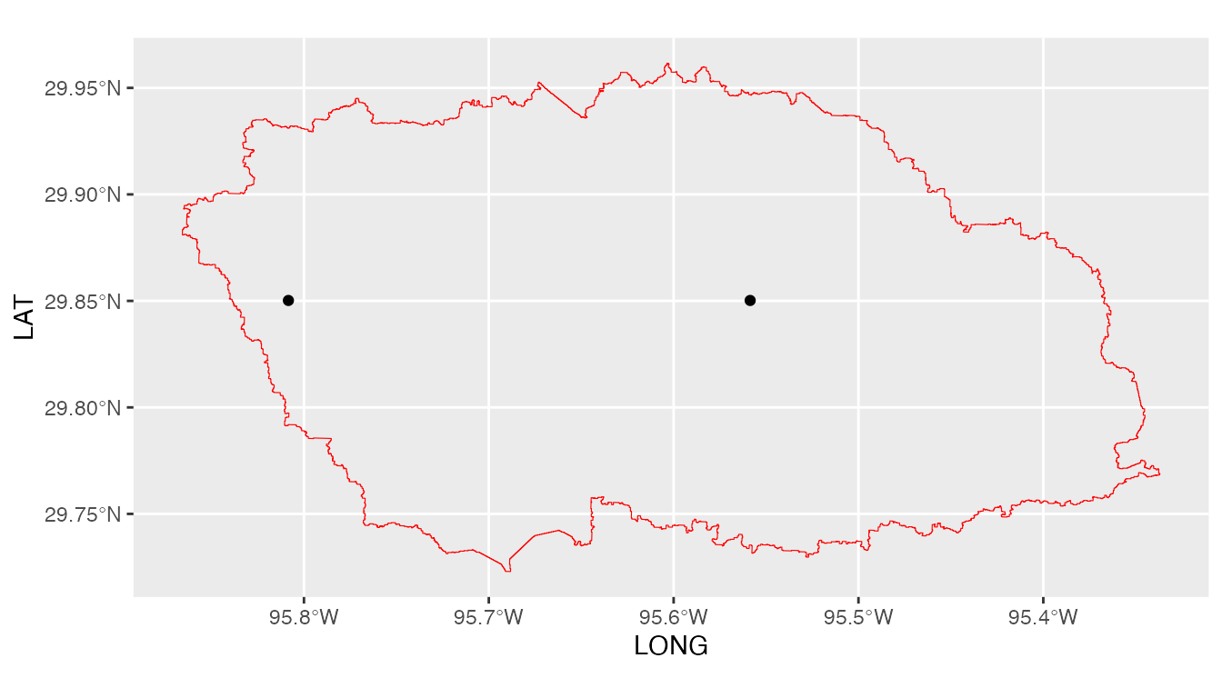

We note here that GLDASwat has given us all the GLDAS data grids that fall within the boundaries of the White Oak Bayou study watershed.

The time series air temperature data stored in the data tables (i.e., 2 tables) can be viewed also. looking at air temperature reformatted data from the first grid point as listed in the air temperature station file is by


GLDASwat.point.data <- system.file('extdata/GLDASwat',
                              'temp345937.txt', 
                              package = 'NASAaccess')
#Reading data records
read.csv(GLDASwat.point.data)
#>                  X20200801
#> 32.1672399902343  23.28843
#> 33.0642431640625  22.76880
#> 33.7442358398437  22.91977

The time series air temperature data has been written in a format that gives daily maximum and minimum air temperature in degrees ‘C’.

Now, let’s examine GPMpolyCentroid.

Using the watershed example:


GLDASpolyCentroid(Dir = "./GLDASpolyCentroid/",
                  watershed = shape_path,
                  DEM = dem_path,
                  start = "2018-08-1",
                  end = "2018-08-3")

Now let’s examine the GLDASpolyCentroid generated outputs

library(ggplot2)
library(tidyterra)
GLDASpolyCentroid.tempMaster <- system.file('extdata/GLDASpolyCentroid',
                              'temp_Master.txt', 
                                package = 'NASAaccess')

GLDASpolyCentroid.table<-read.csv(GLDASpolyCentroid.tempMaster)

#plot
ggplot(shape) + 
  
  geom_spatvector(color='red',fill=NA) +
  
  geom_point(data=GLDASpolyCentroid.table,
             aes(x=LONG,y=LAT)) +
  coord_sf(xlim=c(-96,-95.2),ylim=c(29.7,30))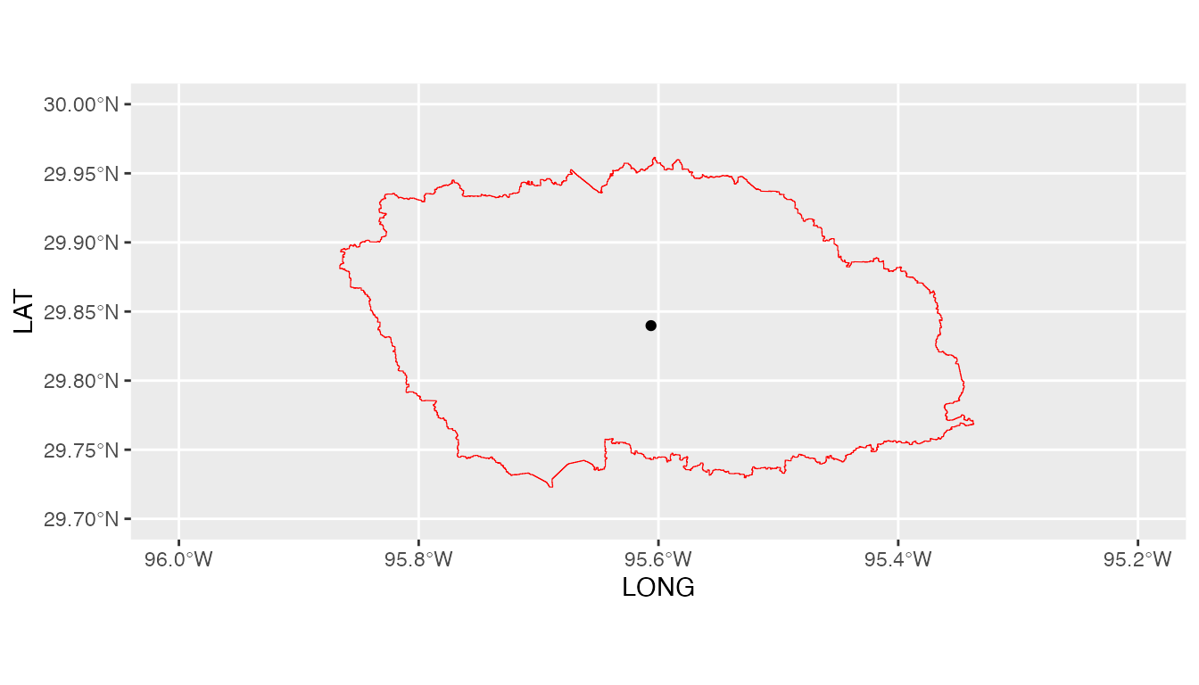

We note here that GLDASpolyCentroid has given us the GLDAS data grid that fall within our specified watershed and assigns a pseudo air temperature gauge located at the centroid of the watershed a weighted-average daily maximum and minimum air temperature data.

Built with

sessionInfo()
#> R version 4.3.0 (2023-04-21)
#> Platform: x86_64-apple-darwin20 (64-bit)
#> Running under: macOS Ventura 13.6.3
#> 
#> Matrix products: default
#> BLAS:   /Library/Frameworks/R.framework/Versions/4.3-x86_64/Resources/lib/libRblas.0.dylib 
#> LAPACK: /Library/Frameworks/R.framework/Versions/4.3-x86_64/Resources/lib/libRlapack.dylib;  LAPACK version 3.11.0
#> 
#> locale:
#> [1] en_US.UTF-8/en_US.UTF-8/en_US.UTF-8/C/en_US.UTF-8/en_US.UTF-8
#> 
#> time zone: America/New_York
#> tzcode source: internal
#> 
#> attached base packages:
#> [1] stats     graphics  grDevices utils     datasets  methods   base     
#> 
#> other attached packages:
#> [1] tidyterra_0.5.1 ggplot2_3.4.4   terra_1.7-55   
#> 
#> loaded via a namespace (and not attached):
#>  [1] sass_0.4.8         utf8_1.2.4         generics_0.1.3     tidyr_1.3.0       
#>  [5] class_7.3-21       KernSmooth_2.23-20 stringi_1.8.3      digest_0.6.34     
#>  [9] magrittr_2.0.3     evaluate_0.23      grid_4.3.0         fastmap_1.1.1     
#> [13] jsonlite_1.8.8     e1071_1.7-14       DBI_1.2.0          purrr_1.0.2       
#> [17] fansi_1.0.6        scales_1.3.0       codetools_0.2-19   textshaping_0.3.7 
#> [21] jquerylib_0.1.4    cli_3.6.2          rlang_1.1.3        units_0.8-5       
#> [25] munsell_0.5.0      withr_2.5.2        cachem_1.0.8       yaml_2.3.8        
#> [29] tools_4.3.0        memoise_2.0.1      dplyr_1.1.4        colorspace_2.1-0  
#> [33] vctrs_0.6.5        R6_2.5.1           proxy_0.4-27       lifecycle_1.0.4   
#> [37] classInt_0.4-10    stringr_1.5.1      fs_1.6.3           ragg_1.2.7        
#> [41] pkgconfig_2.0.3    desc_1.4.3         pkgdown_2.0.7      pillar_1.9.0      
#> [45] bslib_0.6.1        gtable_0.3.4       glue_1.7.0         Rcpp_1.0.12       
#> [49] sf_1.0-14          systemfonts_1.0.5  highr_0.10         xfun_0.41         
#> [53] tibble_3.2.1       tidyselect_1.2.0   rstudioapi_0.15.0  knitr_1.45        
#> [57] farver_2.1.1       htmltools_0.5.7    rmarkdown_2.25     compiler_4.3.0

Ibrahim N. Mohammed

2024-01-13

Basic use

Built with