NASAaccess package has multiple functions such as
GPM_NRT, GPMpolyCentroid and
GPMswat that download, extract, and reformat rainfall
remote sensing data of TRMM and IMERG from NASA servers for grids
within a specified watershed shapefile. The difference between
GPM_NRT and GPMswat functions is the latency
period. The GPMswat function retrieves the IMERG Final Run data which is
intended for research quality global multi-satellite precipitation
estimates with quasi-Lagrangian time interpolation, gauge data, and
climatological adjustment. On the other hand, the GPM_NRT
function retrieves the IMERG near real-time
low-latency gridded global multi-satellite precipitation estimates.
Let’s explore GPMpolyCentroid and GPMswat
functions.
Basic use
Let’s look at an example watershed that we want to examine near Houston, TX:
library(leaflet)
library(ggplot2)
library(terra)
#> terra 1.8.93
#Reading input data
dem_path <- system.file("extdata",
                        "DEM_TX.tif",
                        package = "NASAaccess")

shape_path <- system.file("extdata",
                          "basin.shp",
                          package = "NASAaccess")


dem <- terra::rast(dem_path)


shape <- terra::vect(shape_path)


#plot the watershed data
myMap <- leaflet() %>%
                addTiles() %>%
                fitBounds(-96, 29.7, -95.2, 30) %>%
                addPolygons(lng=terra::crds(shape)[,1],
                           lat=terra::crds(shape)[,2])

myMap
The geographic layout of the White Oak Bayou watershed example used in this demonstration is depicted above. Whiteoak Bayou is a tributary for the Buffalo Bayou River (Harris County, Texas). In order to use NASAaccess we also need a digital elevation model (DEM) raster layer. Let’s see the White Oak Bayou watershed DEM and a more closer look at the study watershed example.
# create a plot of our DEM raster along with watershed (i.e., elevation in meters)

plot(dem,main="White Oak Bayou Watershed with Digital Elevation Model (DEM)")

plot(shape , add = TRUE)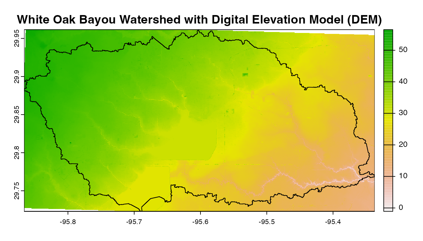
Now, let’s examine GPMswat:
library(NASAaccess)

GPMswat(Dir = "./GPMswat/",
                  watershed = shape_path,
                  DEM = dem_path,
                  start = "2020-08-1",
                  end = "2020-08-3")
Examining the rainfall station file generated by
GPMswat
GPMswat.precipitationMaster <- system.file('extdata/GPMswat',
                                         'precipitationMaster.txt',
                                         package = 'NASAaccess')

# reading GPMswat header file
GPMswat.table<-read.csv(GPMswat.precipitationMaster)

head(GPMswat.table)
#>        ID                 NAME      LAT      LONG ELEVATION
#> 1 2160842 precipitation2160842 29.93337 -95.82337  50.16166
#> 2 2160843 precipitation2160843 29.93337 -95.72340  46.68206
#> 3 2160844 precipitation2160844 29.93337 -95.62343  39.72196
#> 4 2160845 precipitation2160845 29.93337 -95.52346  35.58193
#> 5 2164442 precipitation2164442 29.83343 -95.82337  48.02116
#> 6 2164443 precipitation2164443 29.83343 -95.72340  40.47534

dim(GPMswat.table)
#> [1] 11  5
GPMswat generated ascii table for each available grid
located within the study watershed. There are 11 grids within the study
watershed and that means 11 tables have been generated.
GPMswat also generated the rainfall stations file input
shown above GPMswat.table (table with columns: ID, File NAME,
LAT, LONG, and ELEVATION) for those selected grids that fall within the
specified watershed.
Now, let’s see the location of these generated grid points:
library(ggplot2)
library(tidyterra)
#>
#> Attaching package: 'tidyterra'
#> The following object is masked from 'package:stats':
#>
#>     filter

ggplot(shape) +
      geom_spatvector(color='red',fill=NA) +
      geom_point(data=GPMswat.table,
             aes(x=LONG,
                 y=LAT,
                 fill=ELEVATION),
             shape=21,
             size = 4) +
     scale_fill_gradientn(colours = terrain.colors(7))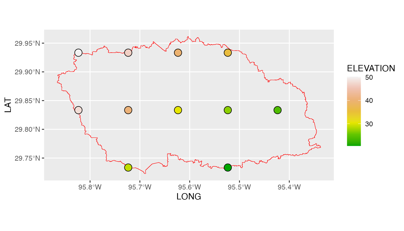
We note here that GPMswat has given us all the GPM data grids that fall
within the boundaries of the White Oak Bayou study watershed. The time
series rainfall data stored in the data tables (i.e., 11 tables) can be
viewed also. looking at reformatted data from the first grid point as
listed in the rainfall station file generated by
GPMswat.
GPMswat.point.data <- system.file('extdata/GPMswat',
                              'precipitation2160842.txt',
                              package = 'NASAaccess')

# reading data records
read.csv(GPMswat.point.data)
#>     X20200801
#> 1 32.22795868
#> 2  1.80884695
#> 3  0.07029478
The GPMswat has generated a ready format ascii tables
that can be ingested easily to the Soil and Water Assessment Tool SWAT model or any other hydrological
model of choice.
Now, let’s examine GPMpolyCentroid.
GPMpolyCentroid(Dir = "./GPMpolyCentroid/",
                  watershed = shape_path,
                  DEM = dem_path,
                  start = "2019-08-1",
                  end = "2019-08-3")
Examining the rainfall station file generated by
GPMpolyCentroid
library(ggplot2)
library(tidyterra)


GPMpolyCentroid.precipitationMaster <- system.file('extdata/GPMpolyCentroid',
                                                    'precipitationMaster.txt',
                                                    package = 'NASAaccess')

GPMpolyCentroid.precipitation.table <- read.csv(GPMpolyCentroid.precipitationMaster)

# plotting

ggplot(shape) +

      geom_spatvector(color='red',fill=NA) +

      geom_point(data=GPMpolyCentroid.precipitation.table,
             aes(x=LONG,y=LAT))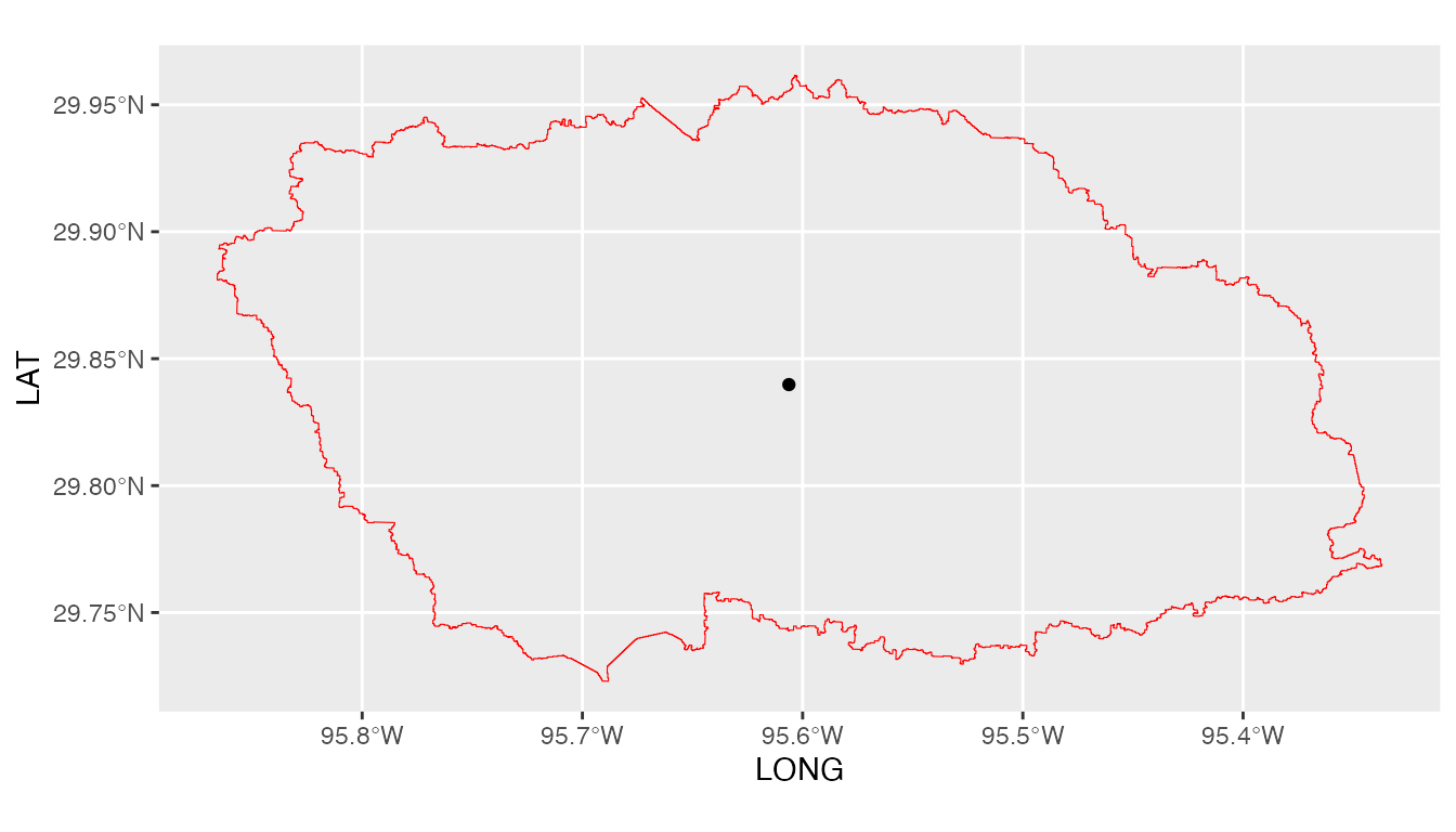
We note here that GPMpolyCentroid has given us the GPM data grid that falls
within a specified watershed and assigns a pseudo rainfall gauge located
at the centroid of the watershed a weighted-average daily rainfall
data.
Let’s examine the precipitation data just obtained by
GPMpolyCentroid over the White Oak Bayou study
watershed.
GPMpolyCentroid.precipitation.record <- system.file('extdata/GPMpolyCentroid',
                                                    'precipitation1.txt',
                                                    package = 'NASAaccess')

GPMpolyCentroid.precipitation.data <- read.csv(GPMpolyCentroid.precipitation.record)

# since data started on 2019-08-01

days <- seq.Date(from = as.Date('2019-08-01'),
                 length.out = dim(GPMpolyCentroid.precipitation.data)[1],
                 by = 'day')

# plotting the precipitation time series

plot(days, GPMpolyCentroid.precipitation.data [,1],
                                    pch = 19, ylab= '(mm)',
                                    xlab = '',
                                    type = 'b',
     main="White Oak Bayou Watershed precipitation (GPM)")
The time series plot above gives the rainfall amounts in (mm) at the centroid of the White Oak Bayou watershed during 2019-August-01 to 2019-August-03.
Last but not least, let’s examine the near real time precipitation
data obtained by GPM_NRT over the White Oak Bayou study
watershed. Remember that the minimum latency for GPM_NRT is
one day. You can experiment this function with yesterday data, nice!
GPM_NRT(Dir = "./GPMswat/",
                  watershed = shape_path,
                  DEM = dem_path,
                  start = "2022-07-1",
                  end = "2022-07-3")
Let’s see one point data record. See that the data starts on July 1, 2022 and ends on July 3rd, 2022.
GPM_NRT.point.data <- system.file('extdata/GPM_NRT',
                              'precipitation2160845.txt',
                              package = 'NASAaccess')

#Reading data records
read.csv(GPM_NRT.point.data)
#>   X20220701
#> 1  2.507078
#> 2  1.148573
#> 3  0.000000
Built with
sessionInfo()
#> R version 4.5.2 (2025-10-31)
#> Platform: aarch64-apple-darwin20
#> Running under: macOS Tahoe 26.3
#>
#> Matrix products: default
#> BLAS:   /System/Library/Frameworks/Accelerate.framework/Versions/A/Frameworks/vecLib.framework/Versions/A/libBLAS.dylib
#> LAPACK: /Library/Frameworks/R.framework/Versions/4.5-arm64/Resources/lib/libRlapack.dylib;  LAPACK version 3.12.1
#>
#> locale:
#> [1] en_US.UTF-8/en_US.UTF-8/en_US.UTF-8/C/en_US.UTF-8/en_US.UTF-8
#>
#> time zone: Asia/Dubai
#> tzcode source: internal
#>
#> attached base packages:
#> [1] stats     graphics  grDevices utils     datasets  methods   base
#>
#> other attached packages:
#> [1] tidyterra_1.0.0 terra_1.8-93    ggplot2_4.0.2   leaflet_2.2.3
#>
#> loaded via a namespace (and not attached):
#>  [1] sass_0.4.10        generics_0.1.4     tidyr_1.3.2        class_7.3-23
#>  [5] KernSmooth_2.23-26 digest_0.6.39      magrittr_2.0.4     evaluate_1.0.5
#>  [9] grid_4.5.2         RColorBrewer_1.1-3 fastmap_1.2.0      jsonlite_2.0.0
#> [13] e1071_1.7-17       DBI_1.2.3          purrr_1.2.1        crosstalk_1.2.2
#> [17] scales_1.4.0       codetools_0.2-20   textshaping_1.0.4  jquerylib_0.1.4
#> [21] cli_3.6.5          rlang_1.1.7        units_1.0-0        withr_3.0.2
#> [25] cachem_1.1.0       yaml_2.3.12        otel_0.2.0         tools_4.5.2
#> [29] dplyr_1.2.0        vctrs_0.7.1        R6_2.6.1           proxy_0.4-29
#> [33] lifecycle_1.0.5    classInt_0.4-11    fs_1.6.6           htmlwidgets_1.6.4
#> [37] ragg_1.5.0         pkgconfig_2.0.3    desc_1.4.3         pkgdown_2.2.0
#> [41] pillar_1.11.1      bslib_0.10.0       gtable_0.3.6       glue_1.8.0
#> [45] Rcpp_1.1.1         sf_1.0-24          systemfonts_1.3.1  xfun_0.56
#> [49] tibble_3.3.1       tidyselect_1.2.1   rstudioapi_0.18.0  knitr_1.51
#> [53] farver_2.1.2       htmltools_0.5.9    labeling_0.4.3     rmarkdown_2.30
#> [57] compiler_4.5.2     S7_0.2.1